Enzo Joly

A market-making strategy for the Bristol Stock Exchange simulator that replaces the baseline market maker's three fixed thresholds with volatility-scaled equivalents and gates entries on multi-signal confluence. The strategy translates Goichi Hosoda's Ichimoku Kinko Hyō philosophy — "no single indicator is reliable alone, but the probability of a meaningful signal rises with confluence" — into limit-order-book microstructure.

Three of Hosoda's five signals appear: Tenkan-sen as a fast EMA (α = 0.10), Kijun-sen as a slow EMA (α = 0.02), and Kumo cloud polarity (τ = EMA_f − EMA_s). A fourth signal — order-book imbalance, OBI = (V_bid − V_ask) / V_total — comes from Cont (2014). The buy condition fires when all four hold simultaneously: best ask has dropped z_b·σ below the fast EMA, cloud is bullish (τ ≥ 0), OBI > θ_OBI, and balance is sufficient. Sell-side evaluates strictly by priority: stop-loss → end-of-session liquidation → profit-take. Volatility is computed online by Welford's single-pass algorithm with a floor at max(σ_Welford, 0.05·|EMA_f|, 3.0).

Parameter selection

The grid evaluates every combination of z_b, z_s ∈ {0.5, 0.75, 1.0, 1.25, 1.5}, z_st ∈ {4.0, 4.5, 5.0, 5.5, 6.0}, and θ_OBI ∈ {−0.1, 0.0, 0.1, 0.2} — 500 cells, 36 trials each, 18,000 simulations. Three metrics agree on the same hotspot: the upper-left quadrant of each heatmap (low z_b, high z_s), deepening as z_st grows.

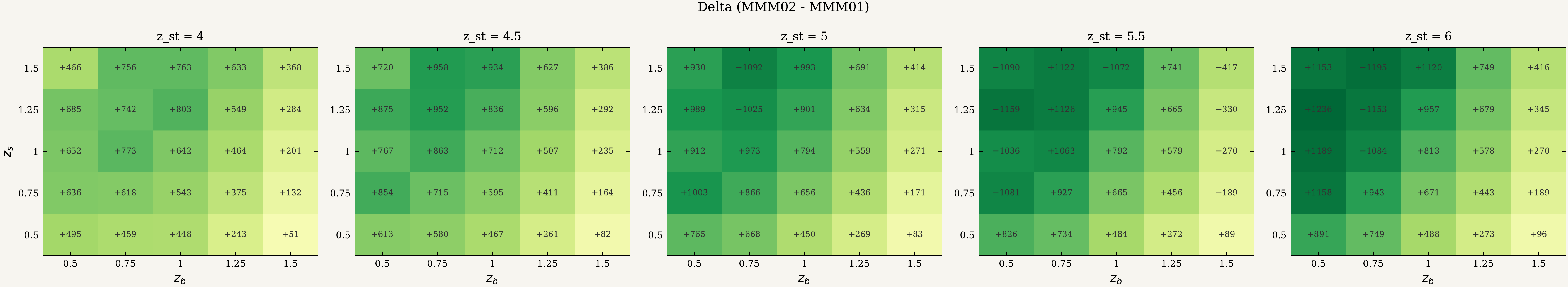
Mean paired delta across the parameter grid — Mean paired delta (MMM02 − MMM01, cents) across the parameter grid at `θ_OBI = −0.1`, sliced by `z_st`. Higher is better; the dark-green corner is where the strategy's edge over the baseline is largest.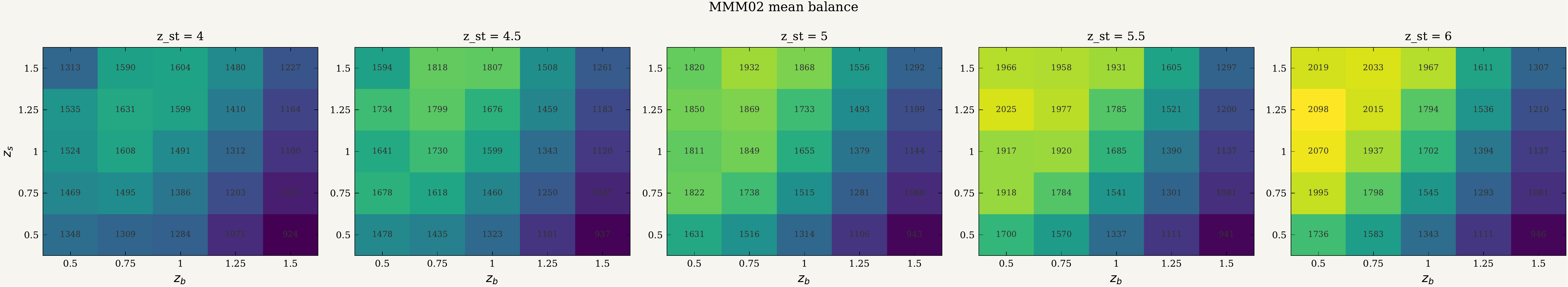

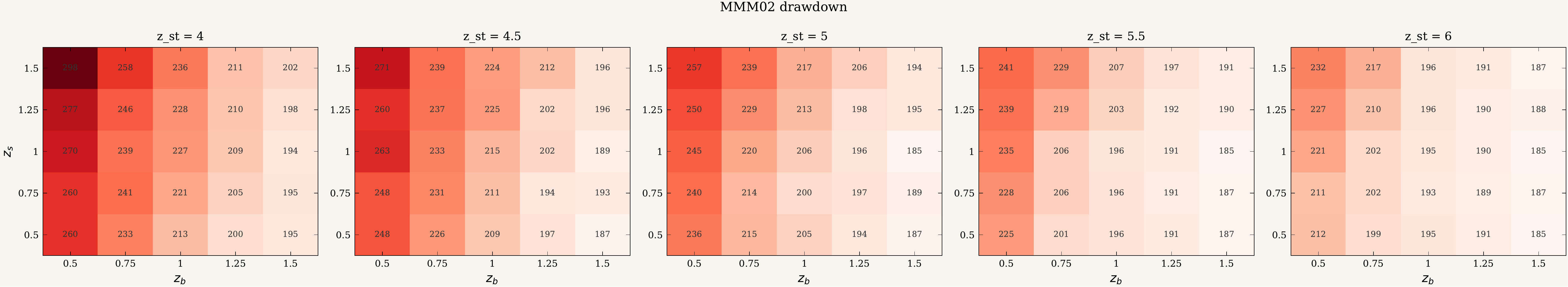
MMM02 mean balance across the parameter grid — MMM02 absolute balance, same slicing. Mean session profitability rather than relative advantage.

MMM02 drawdown across the parameter grid — MMM02 maximum drawdown. Lower is better; the same low-`z_b`, high-`z_s` corner that maximises balance also minimises drawdown.

The selected configuration z_b = 0.5, z_s = 1.25, z_st = 6.0, θ_OBI = −0.1 achieves cell mean delta +$1235.8 with MMM02 winning every cell trial. The top three cells fall within 50 cents of each other; the ranking among the best few is not strongly resolved at 36 trials per cell.

Main results

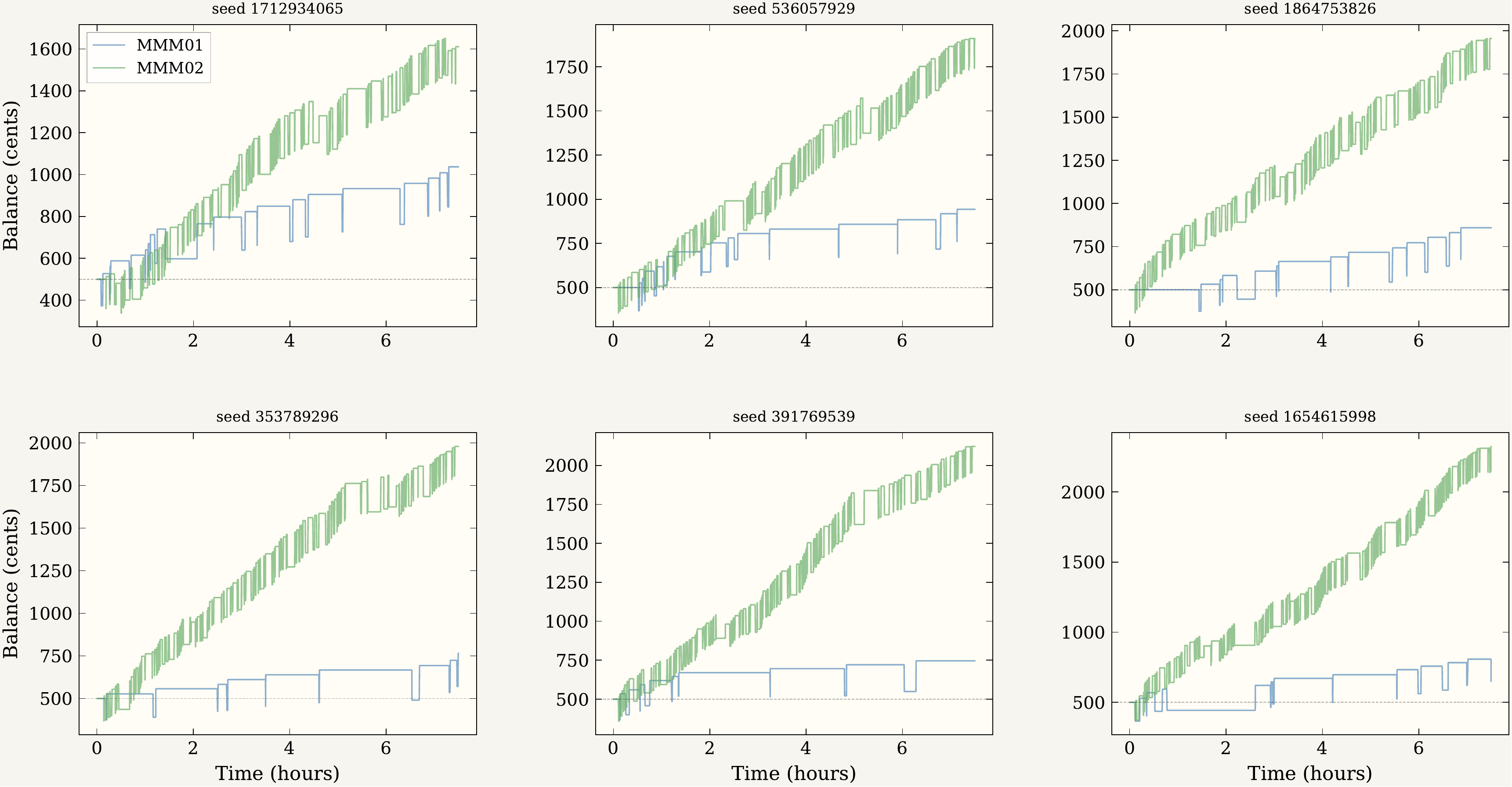
The 120-trial main experiment runs the locked configuration on minute-bar SPY close prices for two consecutive trading days — the second day held out and never used during parameter selection. MMM02 outperformed MMM01 in every paired trial on both offsets. Even the minimum per-trial advantage (+$574 training, +$598 test) exceeded MMM01's typical total session earnings.

Metric	Training		Test (held out)
	MMM01	MMM02	MMM01	MMM02
Balance mean (¢)	871.2	2087.4	879.3	1939.3
Balance SD	108.9	181.2	113.7	182.5
Round-trips (mean)	13.5	115.3	13.8	106.2
Paired delta (mean)	+1216.2 (σ = 219.6)		+1060.0 (σ = 217.9)
Wins	120 / 120		120 / 120

Balance trajectories across six paired sessions — Balance trajectories across six representative paired training sessions. MMM01 (blue) and MMM02 (orange) face identical market conditions within each trial; the gap accumulates monotonically rather than arriving through a late spike.

Behavioural validation

Of 648 training entries and 637 test entries, 100% occurred with τ ≥ 0: the cloud gate is a hard filter, not a soft bias. τ at entry is not clustered at the boundary but distributed several units into bullish territory (median 2.93, mean 3.54 on training data) — robust to perturbation rather than satisfied as a technicality at crossover. Exit breakdown is 86% profit-take, 2% stop-loss, 12% end-of-session liquidation; per-trade win rate 97.5–98.1%; mean hold time around 100 seconds.

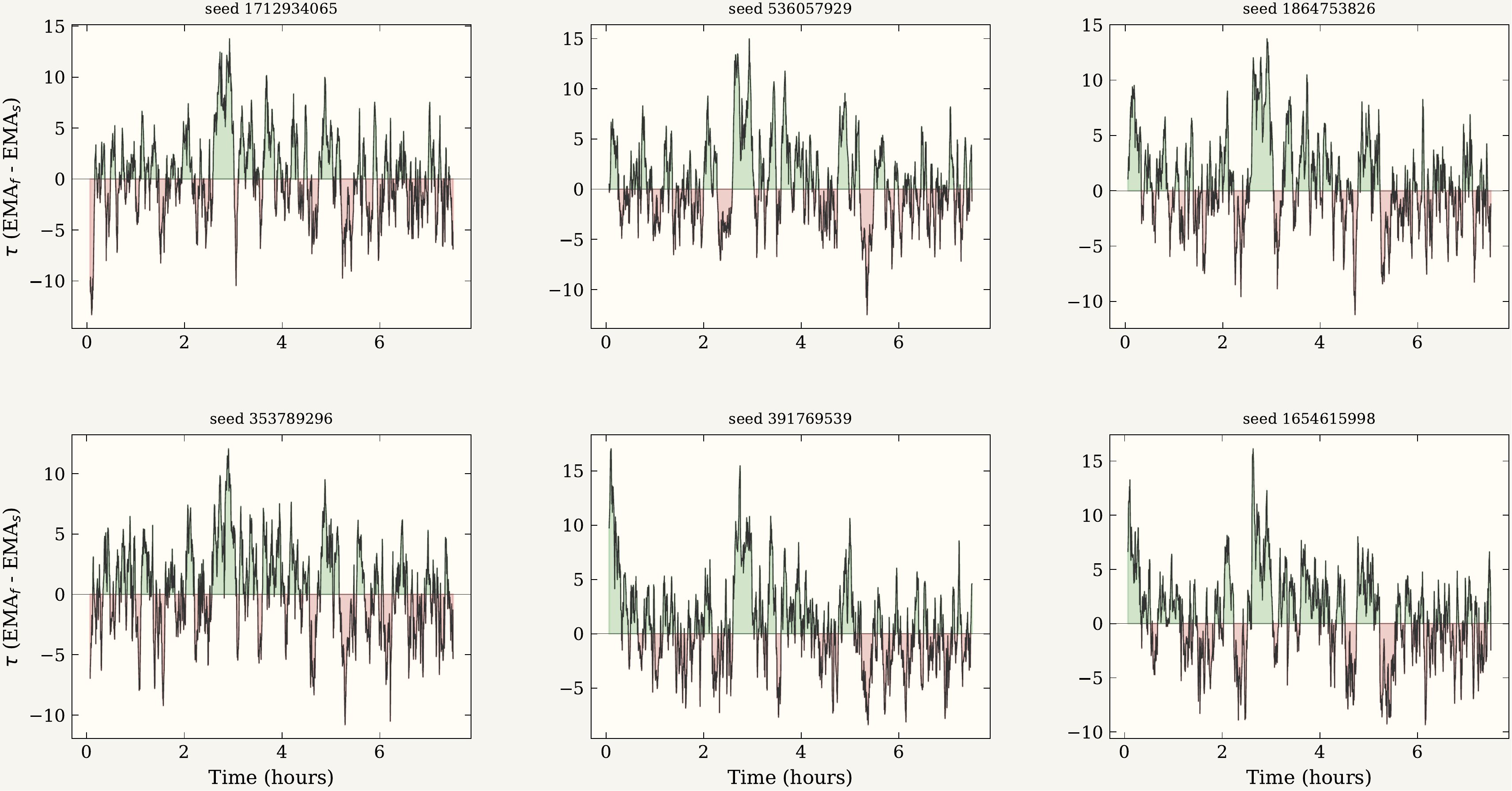
Cloud polarity across six training sessions — Cloud polarity `τ = EMA_f − EMA_s` across six training sessions. Green areas are bullish (`τ > 0`); MMM02 only enters during these intervals.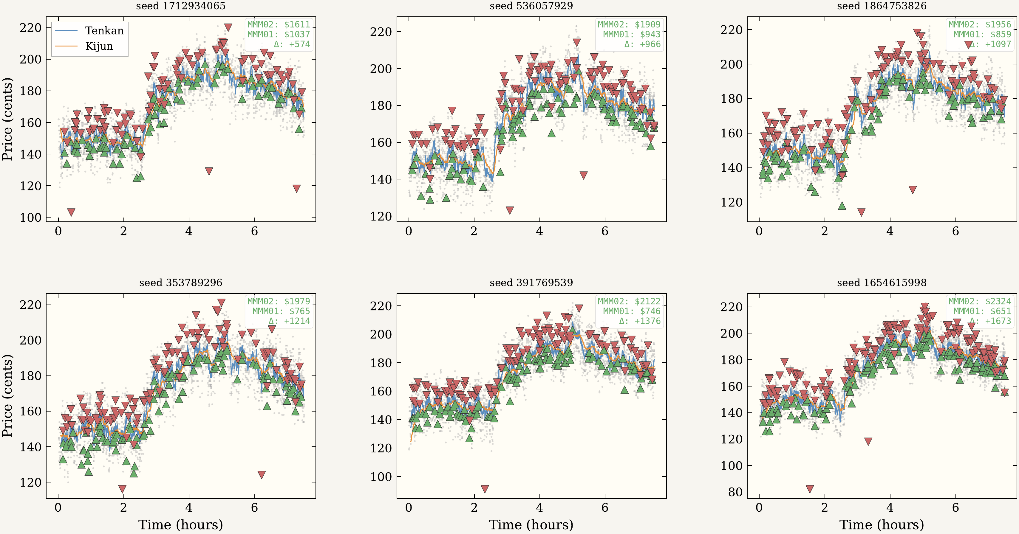

Six training trials at quantile positions of the delta distribution — Six training trials at quantile positions P₀ (worst) through P₁₀₀ (best) of the paired-delta distribution. Grey: transaction prices. Blue: fast EMA. Orange: slow EMA. Green triangles: MMM02 buy signals. Red triangles: sells.

Limitations

The test offset is adjacent to training: one trading day later, with the same starting equity and a similar volatility regime. Mean paired advantage fell roughly 13% across these consecutive sessions, paired Cohen's d_z dropping from 5.54 to 4.86. This is the only variation the experiment probes. Whether the strategy holds on a different week, a different equity, a more bearish regime, or a low-volume session is not addressed by these results. An evaluation across two adjacent days cannot fully separate genuine mechanism from offset-specific overfitting. BSE imposes no transaction costs, which would change everything in a real venue.

StackPython · BSE simulator · Welford's algorithm · Cohen's d_z · Mann-Whitney U · rank-biserial · Nix flake · LaTeX (LNCS).

↑ index

A binary classifier for 12,338 peptide observations described by 385 continuous features, where observations cluster into 652 groups (proteins). With p/n ≈ 0.03 the dataset looks well-conditioned for standard k-fold cross-validation, but observations within groups are not independent: the meaningful ratio is p/g ≈ 0.59, and standard k-fold would split groups across folds, overfitting to within-group patterns and producing performance estimates with no relationship to actual generalisation. The whole pipeline is built around this observation.

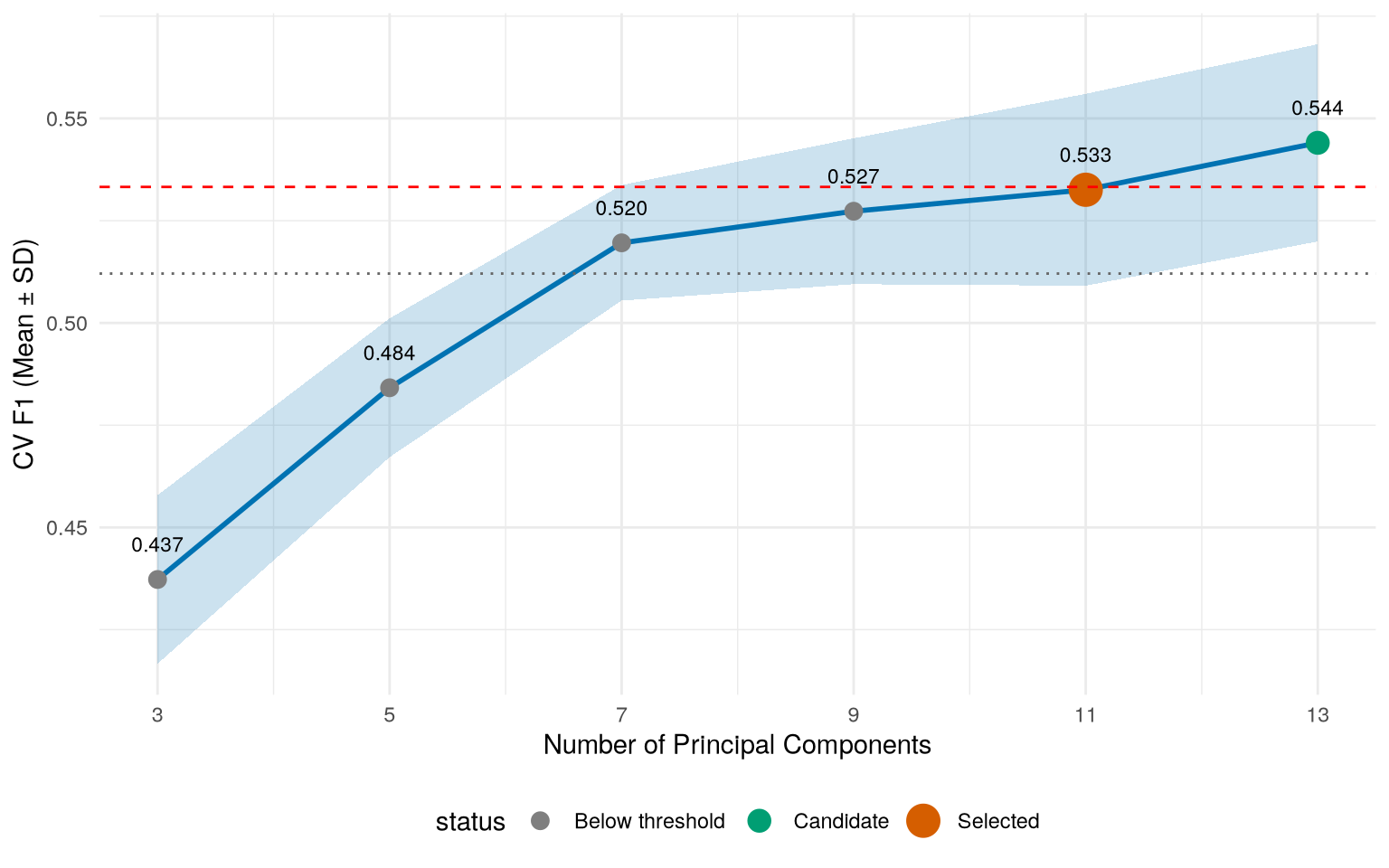
PCA projection showing class overlap — Two-dimensional PCA projection of the standardised feature matrix, coloured by class. The 95% confidence ellipses overlap substantially across both principal axes; no linear hyperplane separates the classes. Class membership emerges from feature interactions, not univariate signal — confirmed by a feature-by-feature discrimination scan in which only one feature exceeded AUC = 0.6, with median AUC = 0.52 across the 385 candidates.

Pipeline

The cleaned dataset splits via group_initial_split() into three partitions where no protein appears in more than one set: 64% training, 16% validation, 20% held-out test. Within training, model evaluation uses group_vfold_cv() so fold assignments respect group boundaries. The preprocessing recipe applies zero-variance removal, median imputation (resilient to the 92% of features with 3×IQR outliers), z-score normalisation (the data spans 11 orders of magnitude), and PCA. The PC count is chosen by ablation rather than a fixed variance target — targeting variance leaks no label information and avoids accidentally chasing F1 in preprocessing.

PC count ablation curve — Cross-validated F1 versus number of principal components retained. The ribbon shows ±1σ across folds; the dashed red line is the one-standard-error threshold from the best configuration. Eleven components (43% cumulative variance) are selected on parsimony.

Architecture comparison

Nested 5-fold cross-validation across three architectures: XGBoost edges Random Forest on F1 at the default 0.5 threshold (0.580 vs 0.546), but Random Forest leads on AUC (0.714 vs 0.696). What survives threshold calibration downstream is ranking quality, not threshold-specific F1, so Random Forest wins on the metric that matters.

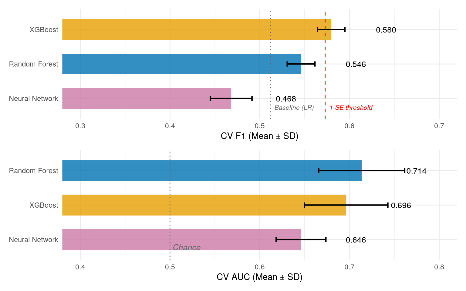
Hyperparameter tuning uses Latin hypercube sampling inside nested 5×3 cross-validation. The F1 landscape is conspicuously flat — performance varies less than 0.02 across the entire grid — so the model is hyperparameter-robust on this problem. Threshold calibration uses the validation set exactly once to shift the decision boundary from 0.5 to 0.4, trading precision for recall.

Test result

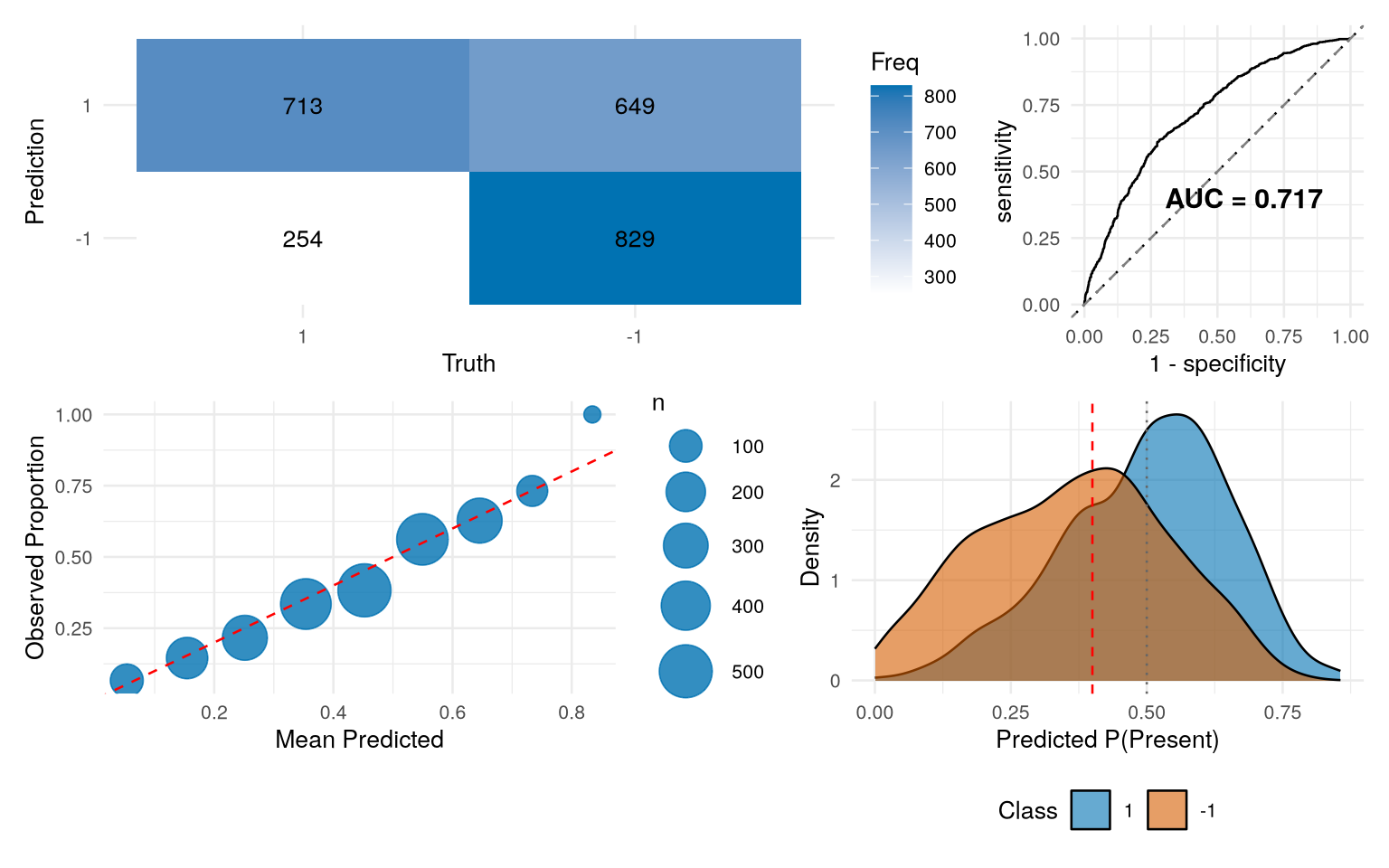
Test set diagnostics: confusion matrix, ROC, calibration, density — Final test-set diagnostics. Top-left: confusion matrix at the calibrated threshold. Top-right: ROC curve, AUC = 0.717. Bottom-left: probability calibration, expected calibration error 0.038. Bottom-right: predicted-probability densities by true class.

Final pipeline: median imputation → z-score normalisation → PCA (11 components) → Random Forest (mtry = 4, min_n = 35, 50 trees, class-weighted). Test F1 = 0.612 with calibrated threshold, AUC = 0.717, calibration error 0.038. Test F1 at the default threshold (0.570) exceeds the unbiased nested-CV estimate (0.544 ± 0.017) by roughly one standard deviation in the favourable direction.

StackR · tidymodels · ranger · xgboost · nnet · pROC · igraph · ggraph · dials · patchwork · R Markdown · renv.

↑ index

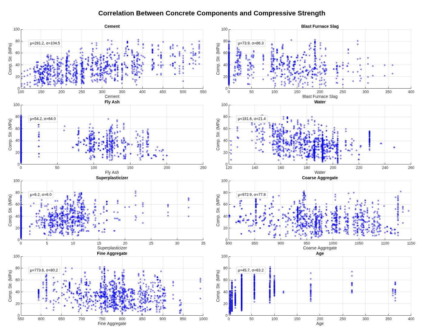
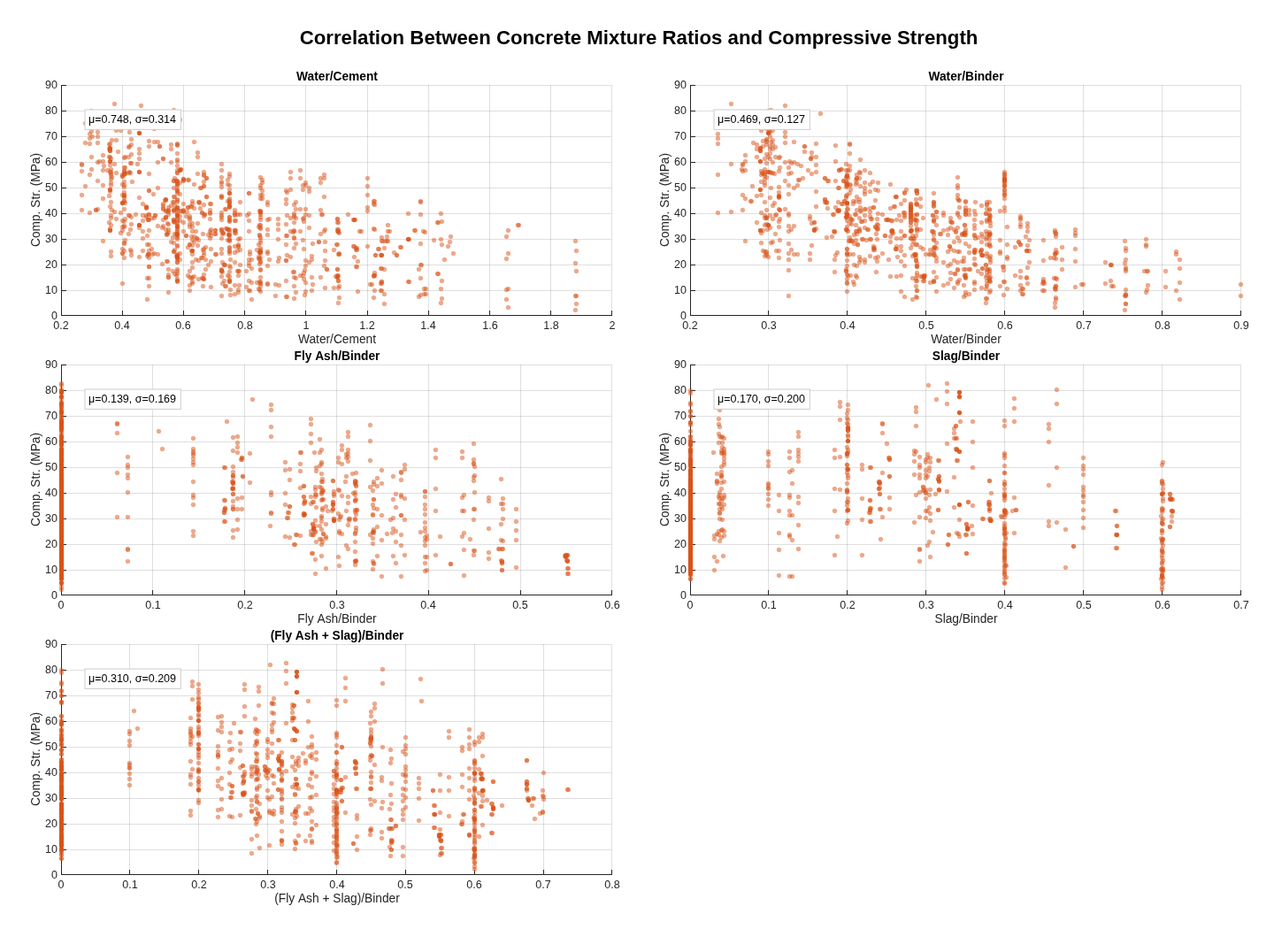
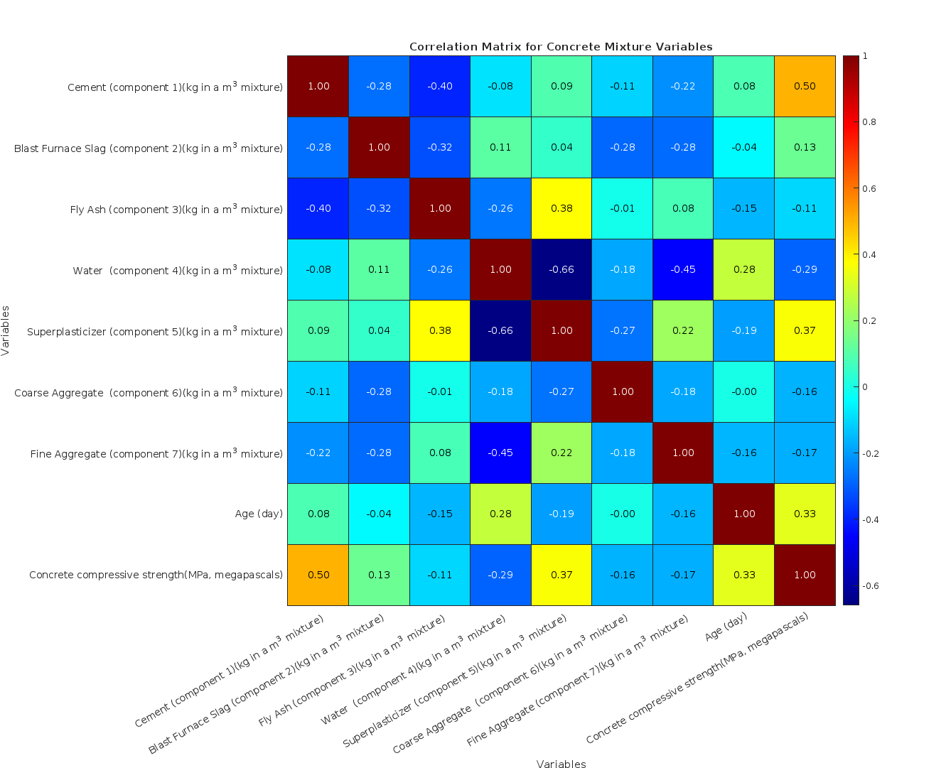
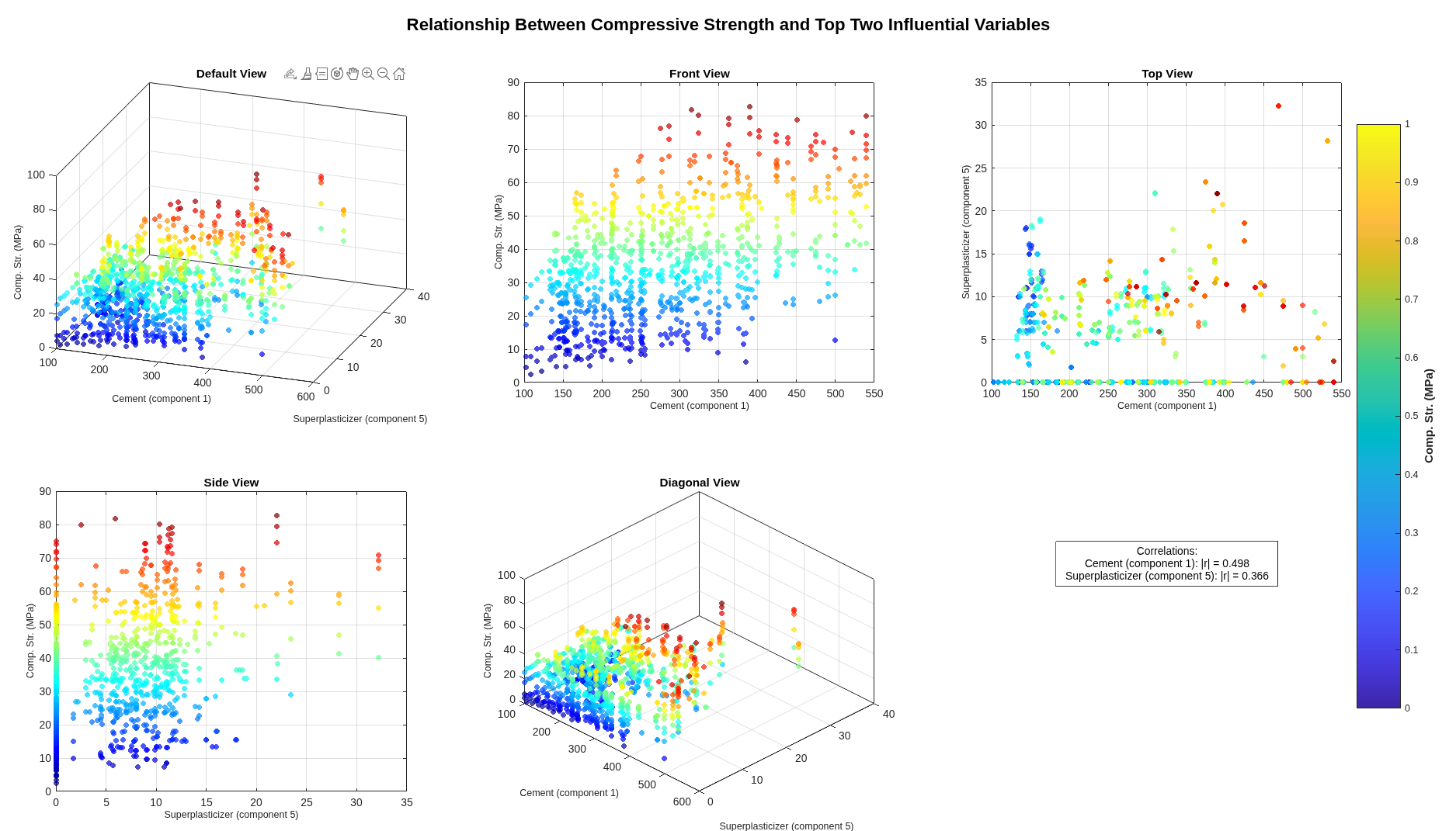
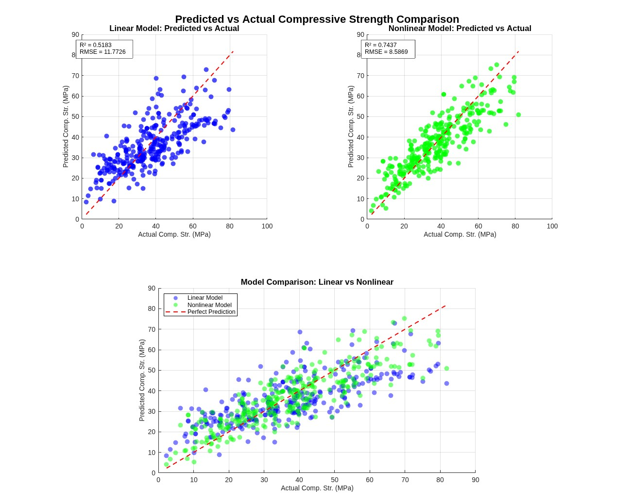
A non-linear regression analysis predicting concrete compressive strength from eight physical mixture components — cement, blast-furnace slag, fly ash, water, superplasticiser, coarse aggregate, fine aggregate, age — using the Yeh (1998) UCI dataset.

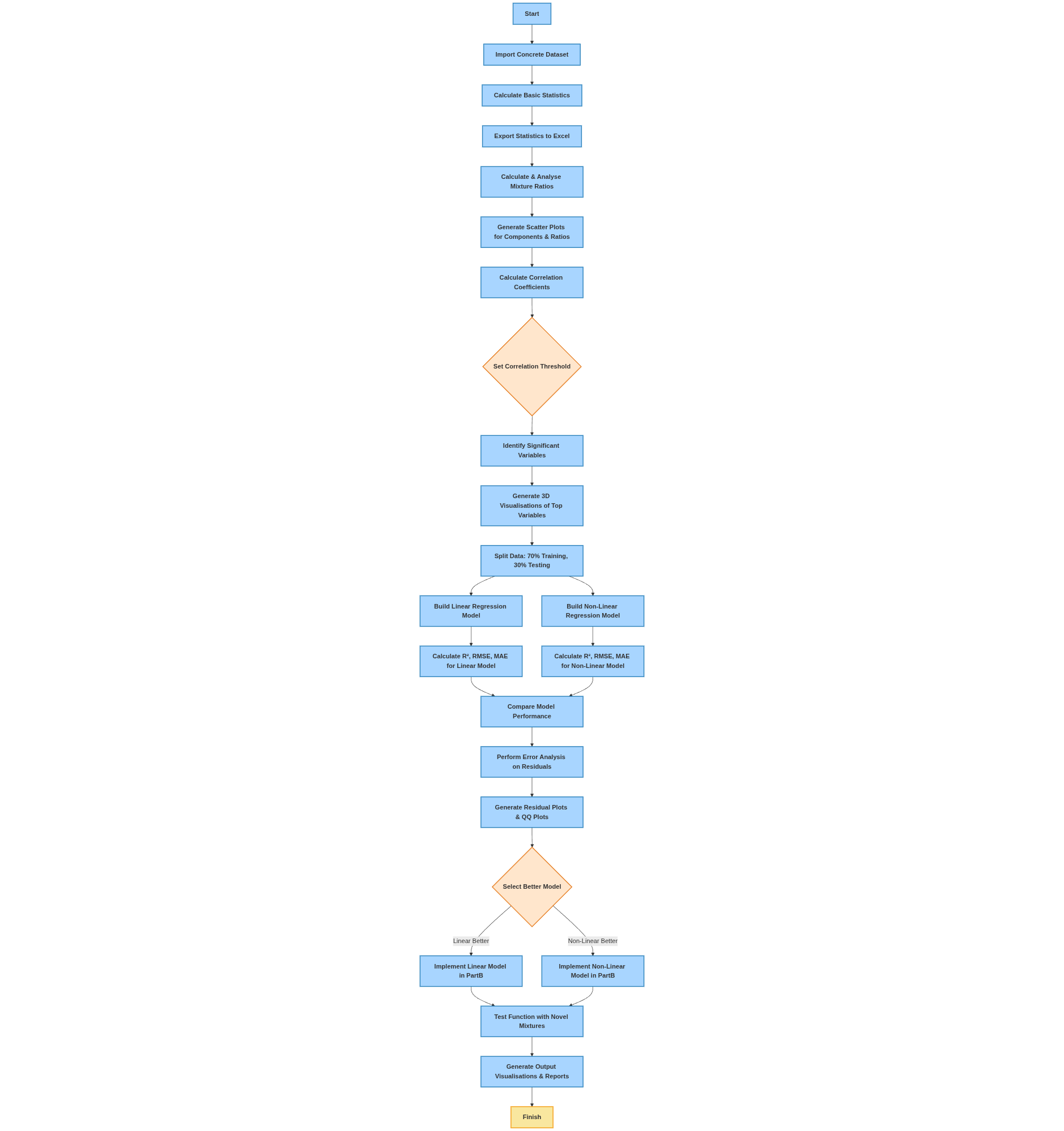
Analysis pipeline flowchart — End-to-end analysis pipeline, from data import through correlation thresholding, train/test split, regression model fitting, error analysis, and selection of the better-performing model for deployment.

Part A executes a complete eight-step pipeline: descriptive statistics with structured Excel export, mixture-ratio calculation (water-to-cement, water-to-binder, fly-ash-to-binder, slag-to-binder, fly-ash-and-slag-to-binder) with explicit zero-division handling that emits warnings rather than silently producing NaN, individual-variable scatter plots, ratio-versus-strength scatters, Pearson and Spearman correlation analysis, 3D visualisation of relationships between top variables, dual linear-and-nonlinear regression model fitting with significant-variable selection at α = 0.05, and rigorous error analysis (R², adjusted R², RMSE, MAPE, residual diagnostics). Each stage writes to its own output directory.

Strength versus each individual component — Compressive strength against each of the eight components, with mean (μ) and standard deviation (σ) annotated per panel. Cement and superplasticiser show the strongest positive correlations; water and fine aggregate the strongest negative.

Strength versus derived mixture ratios — Strength against five derived mixture ratios. Lower water-to-cement and water-to-binder ratios trend toward higher strength, consistent with established concrete-technology principles.

Correlation matrix across components and strength — Correlation matrix across the eight components and compressive strength. Cement (r = 0.50) and superplasticiser (r = 0.37) lead, with age (r = 0.33) and water (r = −0.29) following.

3D scatter of strength vs cement and superplasticiser — 3D scatter of compressive strength against the two top-correlated components — cement (|r| = 0.50) and superplasticiser (|r| = 0.37) — viewed from five angles to make the multi-axis structure legible.

Predicted versus actual strength: linear and non-linear — Predicted versus actual compressive strength on the test partition. Linear model (top-left): R² = 0.518, RMSE = 11.77 MPa. Non-linear with polynomial expansion (top-right): R² = 0.744, RMSE = 8.59 MPa. Bottom: both overlaid against the perfect-prediction diagonal.

Residual analysis: linear vs non-linear model — Residual analysis comparing the linear (blue) and non-linear (green) models. Top: residual scatter against predicted strength. Bottom: residual distribution. The non-linear model's residuals are tighter (σ = 8.58 vs 11.71) and more symmetric around zero (mean 0.58 vs 1.40).

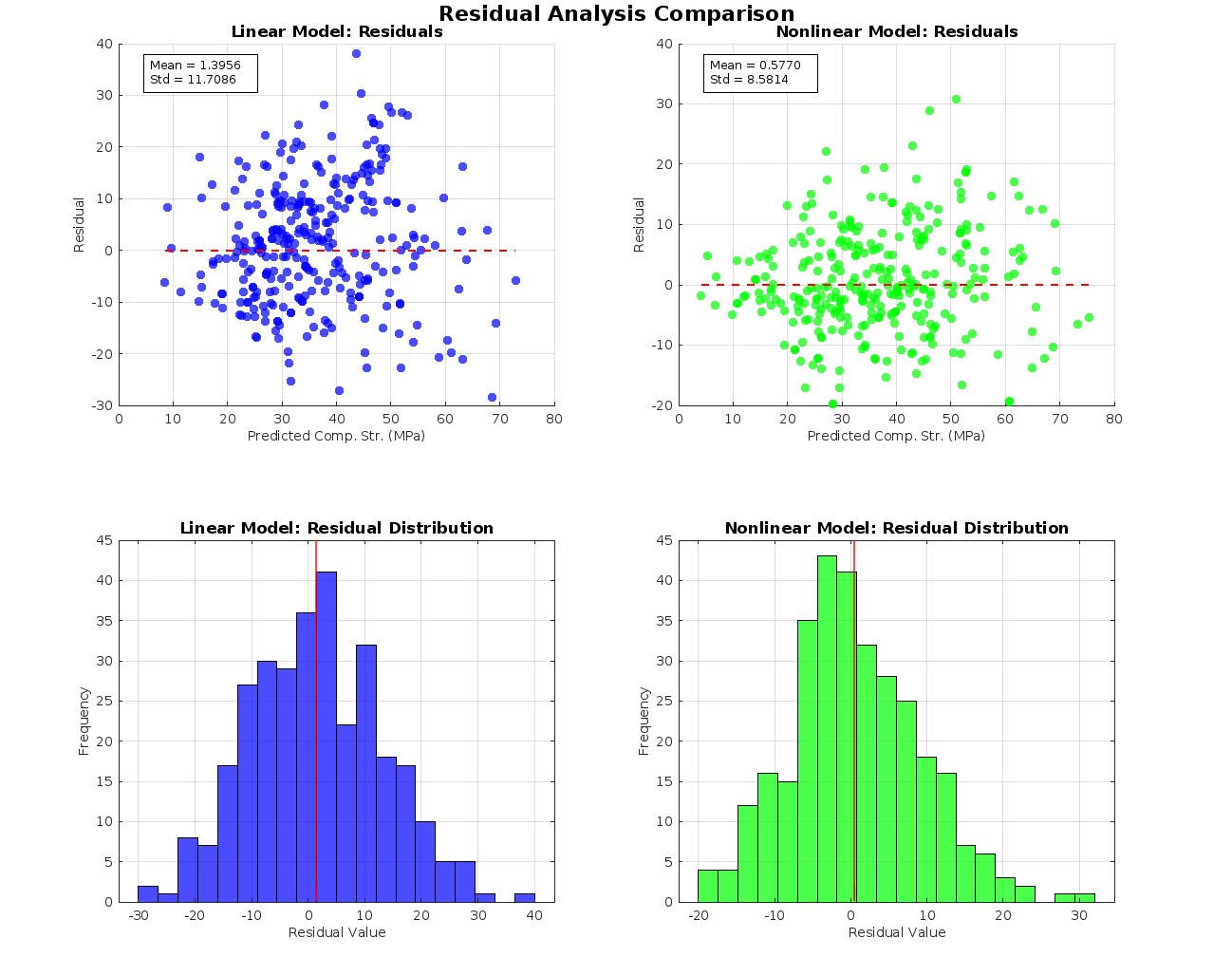
Part B is a deployable prediction function: it takes the eight input components, loads the better-performing model from Part A's output, validates inputs with explicit warnings for division-by-zero edge cases, maps named columns through a containers.Map with case-insensitive contains-fallback for column-name drift between training and inference, and returns both predicted strength and a structured modelInfo describing the model used. Calling PartB() with no arguments produces a help message with a usage example.

StackMATLAB · Statistics & Machine Learning Toolbox · Optimization Toolbox · Excel I/O.

↑ index

An archive-fashion storefront fronted by a character with mood-aware dialogue, typewriter signal events, and a state machine that responds to connection health. Vanilla TypeScript with morphdom for incremental DOM patching, Bun for runtime and bundling, custom service worker for offline detection. Built from scratch — no React, no Next.js, no framework that will be deprecated by 2027.

The architecture treats dialogue as data rather than code: tagged-emotion lines ({ text, emotion: 'sly' | 'pleased' | 'concerned' | 'loss' | …, showName }) are indexed by scene state (idle, addedToCart, removedFromCart, connectionDegraded, connectionLost, connectionRestored), and the typewriter renderer handles per-character animation with skip-on-click. The connection monitor watches both navigator.onLine and active health-check polling; the character's emotional state changes accordingly.

Deploy is a Nix flake app: nix run .#ship compiles the production server to a single Bun binary, patchelfs the interpreter to the standard glibc loader, scps the binary to the production host, and restarts the systemd service. One command, hash-pinned dependencies, no Docker registry, no Kubernetes.

rocksexchange storefront — ロック, the rocksexchange store assistant.

StackTypeScript · Bun · morphdom · Service Workers · WebGL caustics · variable fonts · Nix flake apps · systemd deploy.

↑ index

The TypeScript starter underneath rocksexchange and several smaller things. Small repository — around 1,600 lines including font OFL boilerplate — but every piece is load-bearing.

The build pipeline is the headline. nix run .#build runs four steps: install with frozen lockfile, browser bundle via bun build, server compile to a self-contained bun-linux-x64 binary with the entire static asset tree baked in via Bun's import asset from "./path" with { type: "file" } syntax, and a final patchelf --set-interpreter /lib64/ld-linux-x86-64.so.2 app-bin step to make the Bun-compiled binary use the standard glibc loader rather than the Nix-store loader (which won't exist on the production server). The build verifies the patch took and fails if not. nix run .#ship chains the build with scp app-bin ${remote}:${path}/app-bin && ssh ${remote} "systemctl restart app". One command, hash-pinned dependencies, single-binary deploy.

The connection daemon is the genuinely novel piece. A 200-line ConnectionMonitor class maintains state across CONNECTED / DEGRADED / DISCONNECTED, listens to service-worker messages as the primary signal (50 ms polling from inside the service worker, broadcast to clients via postMessage), and falls back to direct /health polling at 1 Hz from the main thread. Clicking the connection indicator opens a diagnostic panel showing current state, the last ten events with timestamps, latency history, and browser online status.

StackTypeScript · Bun · morphdom · Service Workers · variable fonts · Nix flake apps · patchelf · systemd deploy.

↑ index

An end-to-end BPMN-orchestrated business process for a car repair shop, built on Camunda Zeebe with Spring Boot workers, Stripe and Calendly integrations, and a CSV-backed membership service for discount logic. Multi-service Spring Boot worker, externalised configuration via dotenv, JSON form definitions for human task UIs, BPMN message correlation for inter-process communication.

Two BPMN models exist: a strategic model for high-level business process design (audience: operations management) and an operational model for executable workflow detail (audience: the engine). This separation is exactly the discipline BPMN was designed for and rarely actually maintained in practice. Five JSON forms — onboarding, quote approval, repair cost, test passing, satisfaction verification — provide the human-in-the-loop UI. The Worker class wires Zeebe's @ZeebeWorker annotations to BPMN service tasks, with inner ProcessVariables and MessageNames classes acting as a single source of truth for variable names — avoiding the classic Camunda string-typo footgun.

The accompanying academic deliverable in a sibling repository is approximately 25,000 words of LaTeX across four essays: goal-oriented requirements engineering using iStar 2.0 (a four-actor socio-technical model with strategic dependencies and rationales), strategic BPMN, operational BPMN, and testing methodology with appendix.

StackJava 17 · Spring Boot · Camunda Zeebe · BPMN 2.0 · JSON Forms · Stripe API · Calendly API · Maven · iStar 2.0 · LaTeX.

↑ index

A from-scratch network simulator structured as eleven loosely coupled subsystems: Simulator as top-level orchestrator, SimulationClock as time authority, TopologyManager managing nodes and links, PacketTransmission and Packet for in-flight data, BandwidthUtilization, NetworkCongestion, and NetworkDelay for traffic-state metrics, LoadBalancer for path selection, RoutingEfficiency for graph-level analysis, PacketPrioritizer for QoS handling, ErrorRateModel for packet loss simulation.

The class structure leans on smart-pointer discipline: std::unique_ptr for owned components (the simulator owns its subsystems exclusively), std::shared_ptr for TopologyManager (multiple components consult the topology), std::weak_ptr for back-references from Node to Link to prevent reference cycles in the graph data structure that would otherwise leak memory under topology mutations. The simulator's main loop drives simulateNetworkDynamics() → updateComponentStates() → processPackets() → takeSnapshot() at a fixed timestep with a 300-second default snapshot interval.

Not a discrete-event simulator with a proper event queue, and not integrated with ns-3 or OMNeT++. Standalone — good for learning, but results are not directly comparable to literature.

StackC++17 · smart pointers · STL · header-only domain types · Makefile.

↑ index

A polynomial root-finder handling degrees 1 through arbitrary, dispatching to closed-form solutions where they exist (linear, quadratic, cubic, quartic via Ferrari's method) and falling back to Durand–Kerner numerical iteration for degree ≥ 5 — the threshold imposed by the Abel–Ruffini theorem, after which no general algebraic closed form exists.

The quadratic uses the numerically stable Citardauq form (q = −0.5 · (b ± √Δ); r₁ = q/a; r₂ = c/q) rather than the textbook quadratic formula, avoiding catastrophic cancellation when b² ≫ 4ac. The cubic dispatches across five cases — triple root, depressed cubic, pure cube, three-real-roots via trigonometric method, and Cardano's general formula. The quartic uses Ferrari's resolvent cubic — solve a cubic, factor the quartic into two quadratics, solve each, verify by substitution. The Durand–Kerner iteration starts from initial guesses arranged on a perturbed circle (0.4 · exp(2πik/n + 0.01k)); the small phase offset breaks rotational symmetry that would otherwise cause convergence failure on polynomials with symmetric root distributions.

After finding roots, the code groups them by approximate equality, partitions them into real and complex, identifies conjugate pairs among the complex roots, and reconstructs a factorisation in the form a human would actually write — conjugate pairs collapsed into real-coefficient quadratics rather than displayed as separate (x − (a+bi))(x − (a−bi)) factors.

StackHaskell · Data.Complex · Horner's method · Citardauq · Cardano · Ferrari · Durand–Kerner.

↑ index

A transformer-based ticket classifier built for the UWE service desk. The repository structures around three Jupyter notebooks (training pipeline, inference testing, synthetic data generation via Faker), a Dockerfile for reproducible JupyterLab, and processed datasets combining real service-location data with open-source ticket corpora and Faker-generated subject lines and email bodies. The hybrid synthetic-real approach was deliberate: it allowed public release without exposing real ticket content.

The model is XLNet for sequence classification with the corresponding XLNet tokeniser, fine-tuned on labelled service-category data using PyTorch and HuggingFace Transformers, AdamW optimiser, evaluation through standard pandas/seaborn/matplotlib. The choice of XLNet over BERT is non-trivial: XLNet's permutation language modelling captures bidirectional context without BERT's [MASK]-token train/inference mismatch. For short structured documents like email subject and first-paragraph body, the autoregressive aspect matters less than for long-form text, and XLNet's superior pretrained representations on smaller fine-tuning sets are a defensible architectural choice.

Delivered as a five-person team, with project management and architecture selection (BERT, XLNet, Rasa evaluated before settling on XLNet) leading the engineering work.

StackPython · PyTorch · HuggingFace Transformers · XLNet · Faker · Apache Airflow · Papermill · Docker.

↑ index

A 3D-immersive visual redesign for Harvey Hext Trust, a charity working to support families dealing with child bereavement. 3D models by yours truly. Code pair-programmed by myself and good friend, Adam Smith.

Harvey Hext Trust landing page — The redesigned landing page.

The technical surface is Vite + React 18 + TypeScript on the React Three Fiber + Drei + GSAP stack — the canonical modern combo for declarative WebGL scenes with imperative animation overlays. Component inventory: LondonMarathon for the fundraising CTA, DonateSection, AnimatedTimeline for narrative progression, LoadingManager for asset preloading and progress UI, SponsorsSection, VimeoPlayer for embedded video, SplitSection and Twocolumns3D for layout primitives. State management uses Zustand. Both React Spring and GSAP are present — Spring for object-naturally-settles-into-position cases, GSAP for scripted-sequence-of-beats cases.

The companion documentation repository contains five timeboxes of supervisor and client meeting minutes, two revisions of the Project Initiation Document, risk assessments, external testing documentation, a final presentation, and four formal handover documents covering technical setup, content management, deployment, and AWS considerations.

StackTypeScript · React 18 · React Three Fiber · Three.js · GSAP · React Spring · Zustand · Vite · Nix flake · Bun.

↑ index

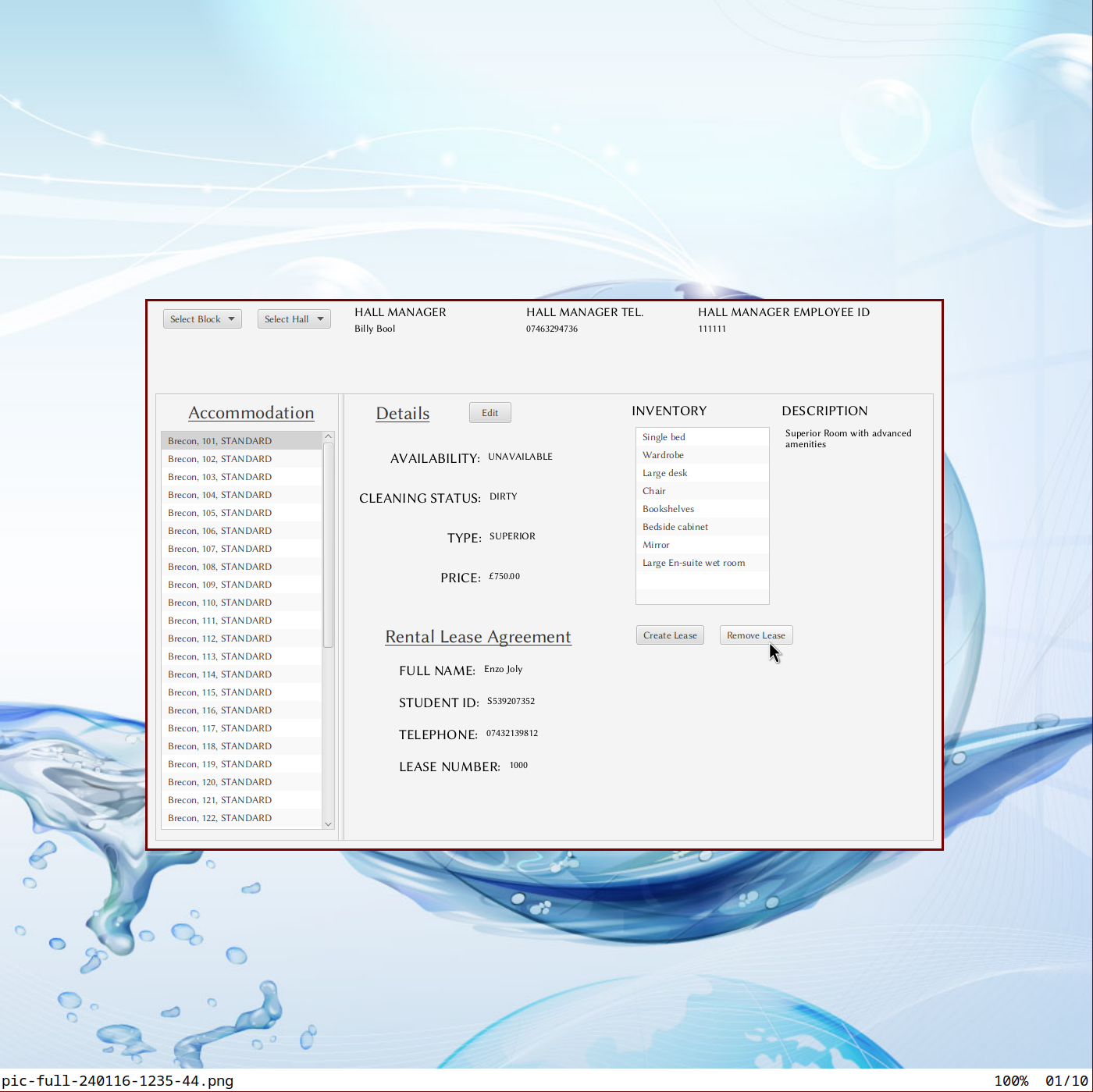
A JavaFX desktop application for student-accommodation administration, designed and delivered single-handedly in two weeks against a brief that synthesised UML modelling with full MVC implementation. The domain model factors cleanly: Person as abstract base, Student extends Person (studentIDNumber, leaseNumber), Manager extends Person (employeeID), Hall containing a list of Accommodation objects and a Manager, RentalAgreement with synchronised auto-incrementing lease numbers (getNextLeaseNumber() synchronised for thread-safe ID generation), and enums for AccommodationType, AvailabilityStatus, CleaningStatus, OccupancyStatus.

The package structure follows convention (uwe.tae.sys.model, uwe.tae.sys.controller, uwe.tae.sys.view), Maven for build, module-info.java for Java 9+ module declarations. The InformationUpdateCallback interface in the controller layer suggests a properly decoupled view-model communication pattern rather than tightly bound JavaFX bindings — model state changes propagate through callbacks rather than direct view manipulation.

HallBook accommodation management UI — HallBook student-accommodation UI in JavaFX, laid out in Scene Builder.

StackJava · JavaFX · Scene Builder · FXML · Maven · Java Modules · MVC · UML.

↑ index

A 3D underwater acoustic propagation model evaluating whether sea-ice events in the Bransfield Strait near Elephant Island are detectable at hydrophone-deployable ranges. The solver implements the parabolic-equation method of Lin et al. (2013) in cylindrical coordinates, evaluated by split-step Fourier on GPU through CuPy and cuFFT. Every layer beneath the solver is grounded in published acoustical oceanography: Mackenzie (1981) for sound speed from temperature/salinity/depth, Ainslie–McColm (1998) for frequency-dependent absorption, Wenz (1962) for ambient noise, Eckart (1953) for surface scattering, Feit–Fleck (1978) for the operator-split propagator.

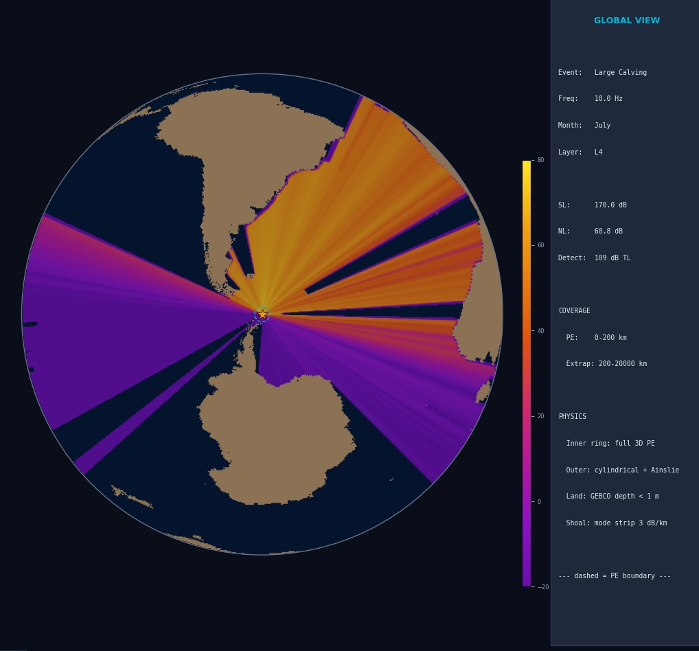
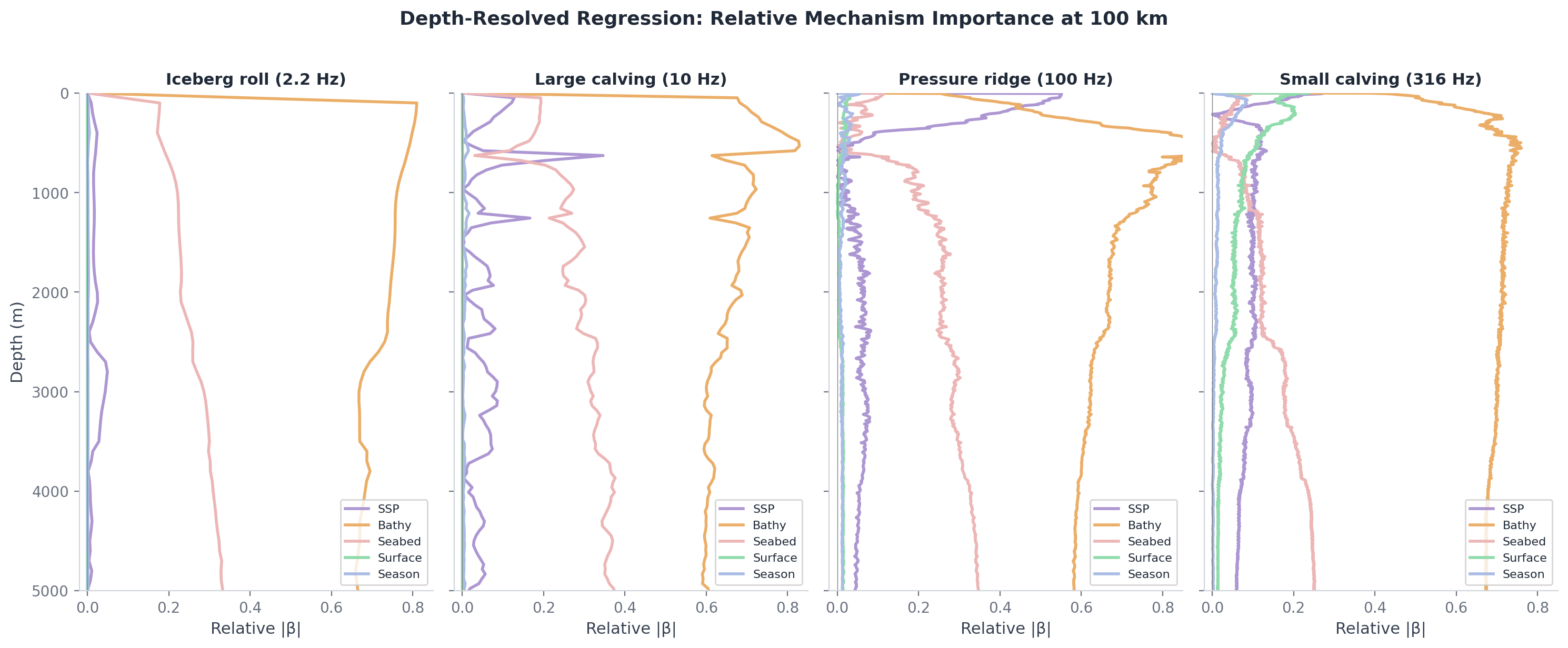
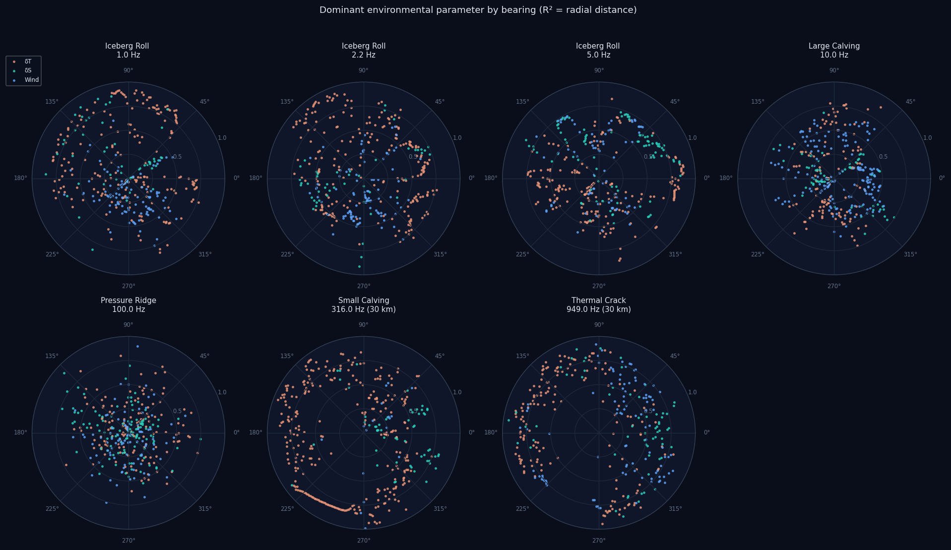
Orthographic global propagation view — Orthographic global projection from the Bransfield Strait source. Inner ring is the full parabolic-equation solver from 0–200 km; outer ring extrapolates cylindrically with Ainslie–McColm absorption out to 20,000 km. Shown: large calving (10 Hz, July, source level 170 dB, detection threshold 109 dB TL).

The experimental design uses five additive sensitivity layers — Pekeris waveguide, then realistic sound speed profile, then bathymetry, then seabed, then surface roughness — running the same algorithm across each. The difference in transmission loss between consecutive layers isolates each physical mechanism's contribution. A polynomial chaos expansion via chaospy and Sobol indices via SALib quantify uncertainty across four parameters (wind speed, ice concentration, sediment properties, channel depth).

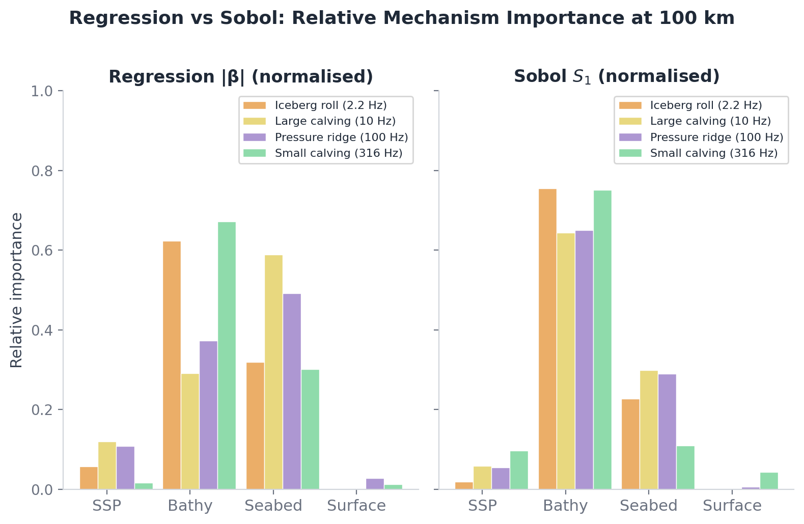
Regression beta vs Sobol S1 attribution — Sensitivity attribution by two methods at 100 km. Left: normalised regression coefficients |β| from a linear model on log-TL. Right: first-order Sobol indices S₁ from polynomial chaos. Both rank bathymetry as the dominant mechanism across all four event types; the methods diverge on the secondary contributor — regression weights seabed properties more, Sobol distributes the remainder more evenly.

Five ice event types span 2 to 3000 Hz: iceberg roll (2.2 Hz, 158 dB source level), large calving (10 Hz, 170 dB), pressure ridge (100 Hz, 155 dB), small calving (316 Hz, 145 dB), thermal crack (949 Hz, 130 dB). Each has source spectrum, depth, and bandwidth grounded in the cryoseismology literature. Twelve months of seasonal variation come from real datasets: GLORYS12V1 monthly T/S, ERA5 hourly winds, NSIDC daily sea-ice concentration, GEBCO 2025 bathymetry, Dutkiewicz (2015) sediment census.

Plan-view geographic transmission-loss overlay — Plan-view transmission-loss overlay across the study area, with detection contours referenced to the ambient-noise floor.

Range-depth waveguide cross-section at a user-selected bearing, showing transmission loss as a function of range and depth through the water column.

Depth-resolved mechanism importance at 100 km, for four ice event types spanning 2.2–316 Hz. Curves show normalised regression coefficients for sound-speed profile (SSP), bathymetry, seabed properties, surface scattering, and seasonal variation. Bathymetry dominates at all depths and frequencies; seabed contribution rises with frequency.

Dominant environmental parameter by bearing across seven ice-event configurations. Each polar plot shows which input — temperature anomaly (δT), salinity anomaly (δS), or wind speed — explains most of the local variance in transmission loss along that bearing. Radial distance is R².

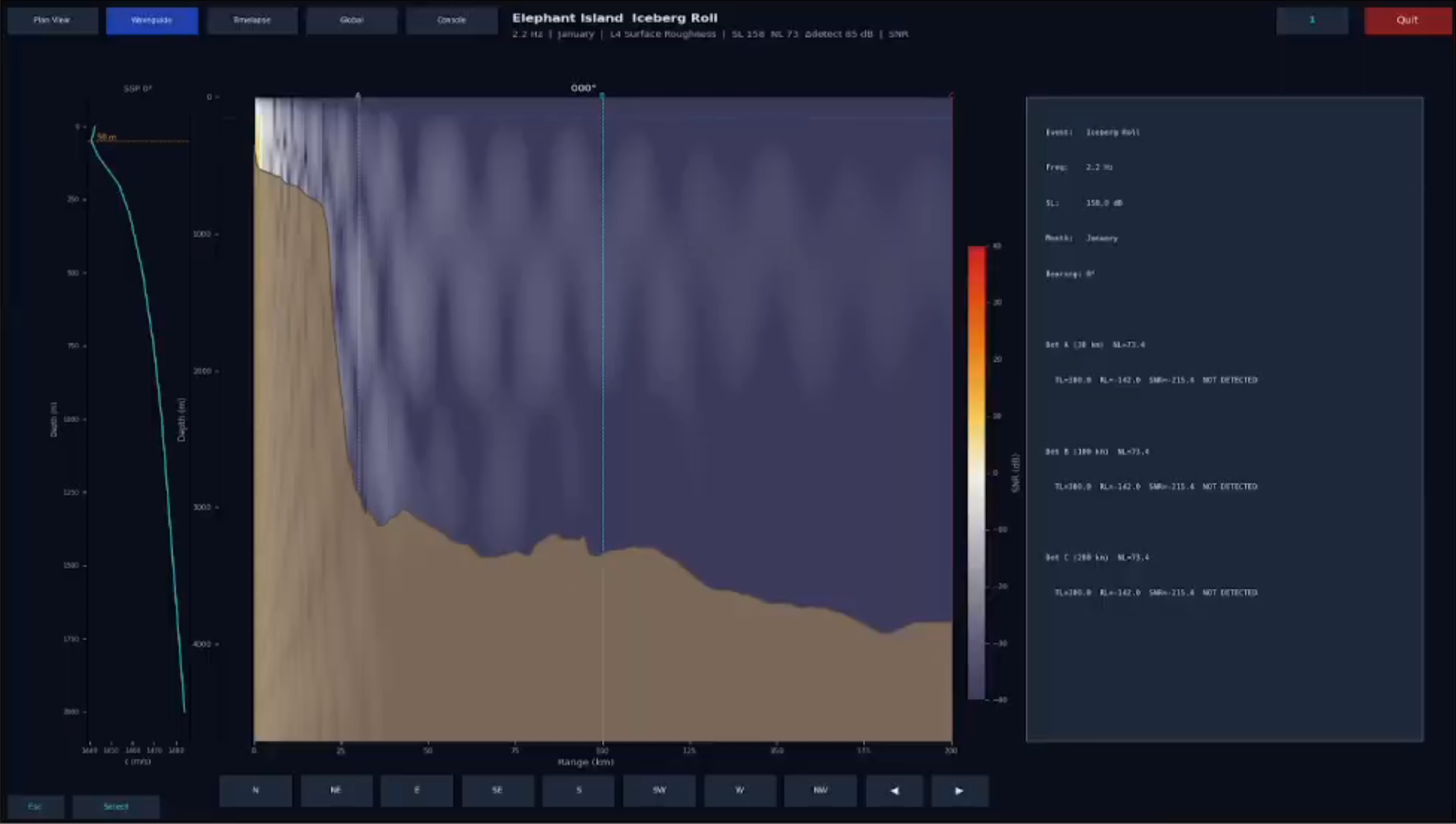
The viewer is a 2,388-line PyQt6 + matplotlib application with five tabs: plan-view geographic overlays, range-depth waveguide cross-sections at user-selected bearings, time-domain pulse propagation reconstructed by inverse FFT, an orthographic global projection extrapolated through real bathymetry, and an interactive console for TL ring queries, detection contours, and Sobol attribution. The Nix flake provides two devShells — a default one without GPU dependencies for the viewer and tests, and a precompute shell with the CUDA stack for actual computation. 172 pytest tests pass.

StackPython 3.12 · CuPy + cuFFT (CUDA 12) · chaospy · SALib · xarray + netCDF4 · matplotlib + PyQt6 · pytest · Nix flake.

↑ index

Ten architecture: CLI, DSL processing, pure core, effect layer — System architecture: CLI through the DSL processing layer, the pure core, and the effect layer.

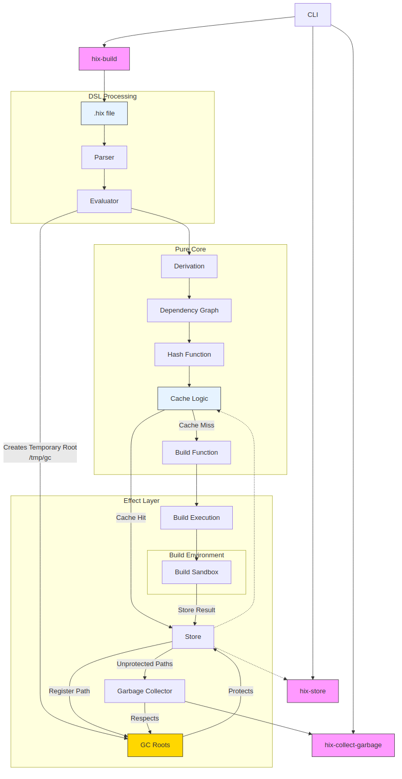
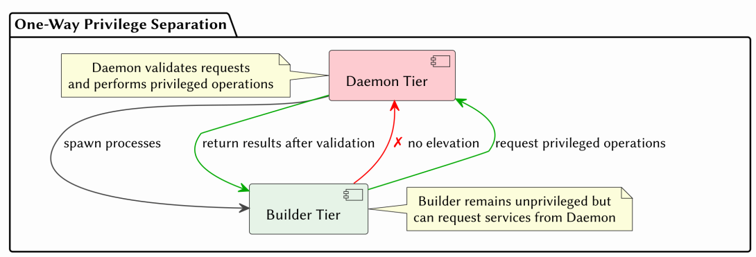
A Nix-inspired build system whose core invariants — phase separation, privilege separation, and content-addressed storage — are enforced statically by the Haskell type system rather than at runtime. The build monad TenM is parametrised by two orthogonal phantom types: Phase (Eval / Build) and PrivilegeTier (Daemon / Builder). Operations that conflate the eval and build phases — Nix's import-from-derivation pathology, for instance — fail to compile. Operations that attempt privilege elevation from an unprivileged builder context fail to compile. There is no escape hatch.

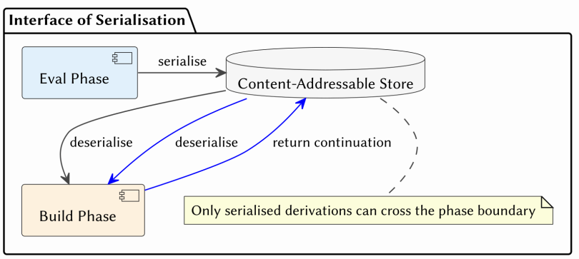
One-Way Privilege Separation between Daemon and Builder tiers — One-Way Privilege Separation.

The architecture follows Dolstra's purely functional deployment model: derivations are immutable build descriptions, store paths are SHA-256 of inputs, content verification happens on every read. Three build strategies are first-class — applicative for parallelisable derivations with statically known dependencies, monadic for sequential builds where structure unfolds dynamically, and return-continuation for multi-stage builds that emit subsequent derivations through $TEN_RETURN_PATH. The last is a generalisation of NixOS RFC#40.

The monad transformer stack (ReaderT BuildEnv → StateT (BuildState p) → ExceptT BuildError → IO) provides clean separation of configuration, mutable build state, error propagation, and effects. Singletons (SPhase, SPrivilegeTier) bridge type-level constraints to runtime dispatch, and type families (CanAccessStore, RequiresDaemon) make capability requirements part of function signatures rather than runtime checks. The "Interface of Serialisation" enforces that only serialised derivations cross the phase boundary.

Interface of Serialisation between Eval Phase, Content-Addressable Store, and Build Phase — Interface of Serialisation.

The dissertation reported eleven of twenty-two functional requirements satisfied at submission. Every requirement other than the CLI is now satisfied: the test suite passes, the daemon and builder protocols work end-to-end, the privilege wall holds against the sandboxing tests. The remaining gap is the user-facing surface — parser and command-line interface — currently in progress.

StackHaskell · GHC 9.8.2 · Cabal · Cryptonite · STM · GADTs · Type Families · Singletons · QuickCheck · HSpec · Nix.

↑ index